SOL Playing Techniques Dataset

A subset of the Studio-on-line dataset labelled according to a taxonomy periodic modulation playing techniques introduced in Wang et al. (2023) [1].

The data consists of 5 possible playing techniques, from 11 distinct musical instruments.

Techniques: ['vibrato', 'trill', 'tremolo', 'bisbigliando', 'flatterzunge']

11 instruments: ['Flutes', 'Strings', 'Horns', 'Trumpets', 'Saxophones', 'PluckedStrings', 'Tubas', 'Oboes', 'Trombones', 'Clarinets', 'Bassoons']

modulation technique  bisbigliando  flatterzunge  tremolo  trill  vibrato
subset                                                                   
test                            61           318      515    216       41
training                       169           905     1513    616      112
validation                      56           300      502    203       37

subset
test          1151
training      3315
validation    1098

Visualizing the playing techniques

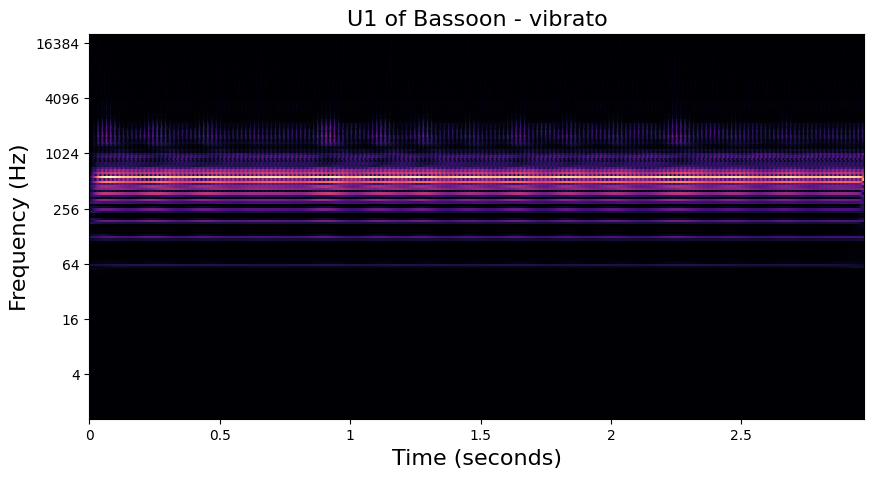
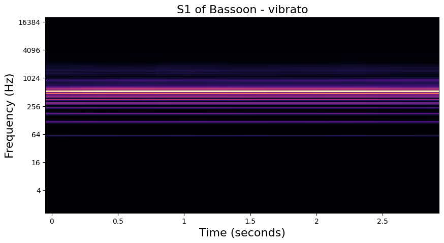
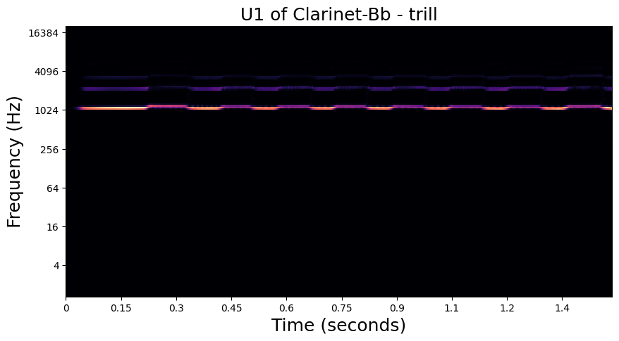
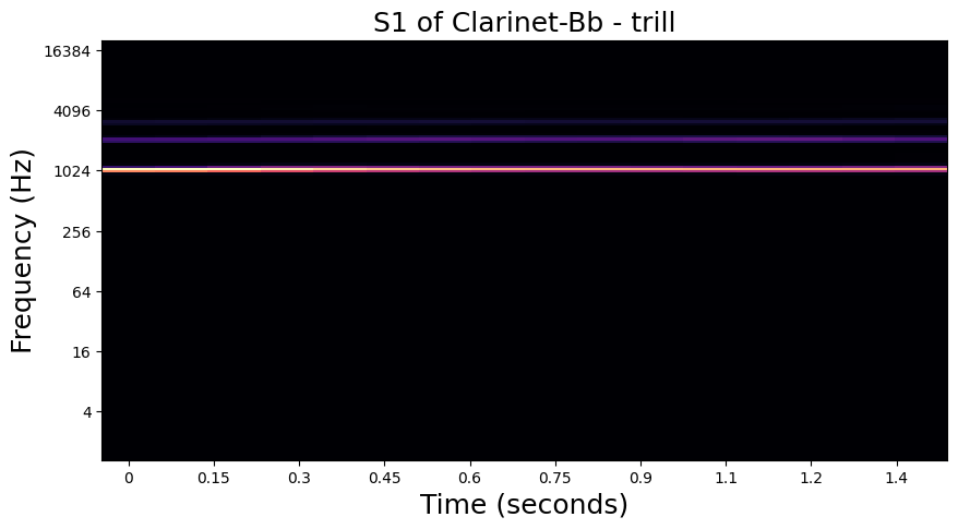
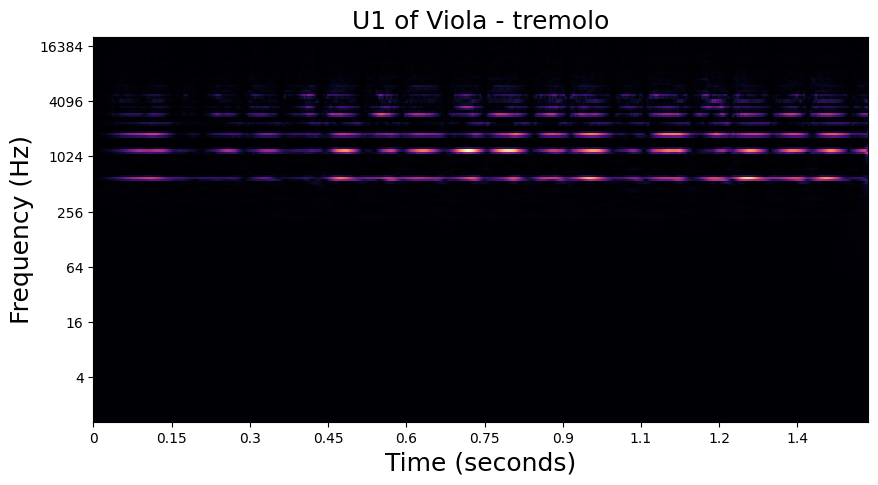
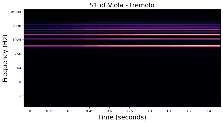
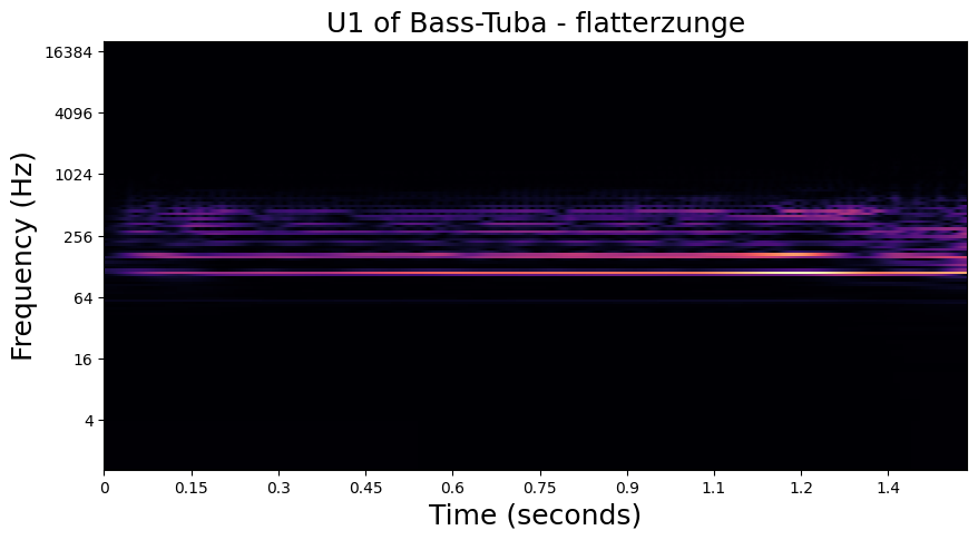
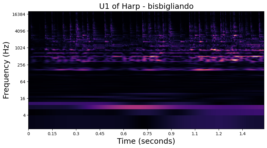
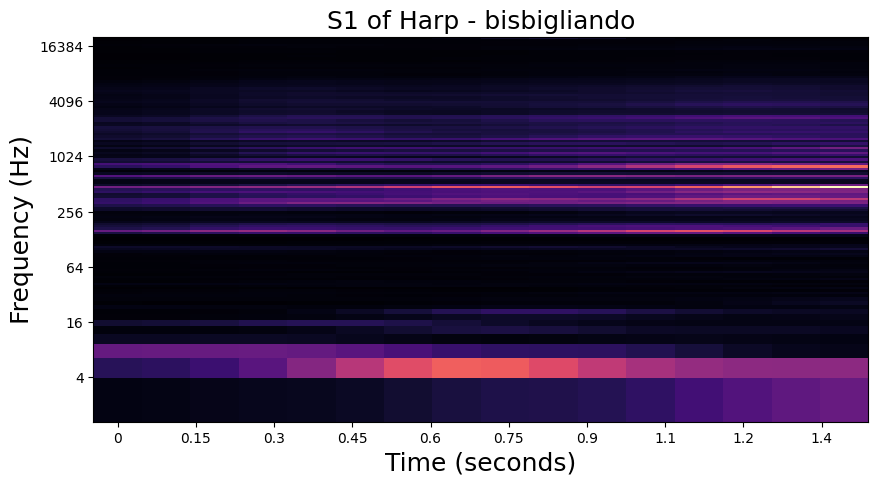
In the examples below, we visualize the \(U_1\) and \(S_1\) of one of each playing technique in the dataset. Importantly, we see that the modulation patterns in \(U_1\) are lost to the averaging operation in \(S_1\). In the notebook in the following section, we will see how these high frequency modulations are recovered in \(S_2\).

Vibrato - Bassoon

Trill - Clarinet

Tremolo - Viola

Flatterzunge - Bass Tuba

Bisbigliando - Harp

Feature extraction

We pre-extract the features offline: CQT with nnAudio and time scatttering / JTFS with kymatio. A numpy array per audio example can be found in SOL_0.9_HQ-PMT/{feature}. We slice the first \(2^{16}\) samples (1.5 seconds) of each audio example. We refer the reader to the following Github repository for the feature extraction codebase.

CQT

    "cqt": {
        "n_bins": 144,
        "bins_per_octave": 16,
        "hop_length": 512,
        "global_avg": False
    }

The resulting CQT has 144 frequency bins and 129 temporal frames. There’s no lowpass filter applied across the CQT’s temporal dimension.

Scattering1D

    "scat1d": {
        "shape": (2**16, ),
        "Q": (12, 2),
        "J": 12,
        "global_avg": False
    },

Time scattering and JTFS give us 16 temporal frames since our hop size is 2**J (2**16 / 2**12). The larger we set T (default 2**J), the more we impose invariance to time-shifts in both spectral shape and spectrotemporal modulations. Time-shift invariance is a useful property, particularly for periodic modulations.

We construct the Scattering1D filterbanks with a maximum scale of J=12 (# octaves). We use 12 and 2 filters per octave in the first and second-order filterbanks respectively. we average over a temporal support of 2**J.

TimeFrequencyScattering

    "jtfs": {
        "shape": (2**16, ),
        "Q": (12, 2),
        "J": 12,
        "J_fr": 3,
        "Q_fr": 2,
        "F": 12,
        "T": 2**13,
        "global_avg": False
    }

We construct the TimeFrequencyScattering temporal filterbanks with a maximum scale of J=12 (# octaves). We use 12 and 2 filters per octave in the first and second-order temporal filterbanks respectively. We average over a temporal support of 2**J and frequential support of Q / F = 1 octave.. The frequential filterbank has its own set of parameters. We use J_fr=3 octaves, with Q_fr = 2 filters per octave. As for time-shift invariance, we can impose frequency transposition invariance with JTFS, by setting F, where transposition invariance is achieved over Q / F octaves. Periodic modulations are invariant to frequency transpositions. In accordance with common fate principles of auditory grouping, the harmonics produced by an instrument will follow congruent spectrotemporal modulation envelopes.

References

1. “Explainable Audio Classification of Playing Techniques with Layer-wise Relevance Propagation” by Changhong Wang et al

2. changhongw/examod Studio-on-Line dataset PMT split.