Nearest Neighbors Regression of Synth Parameters

As a quantitative supplement to the visualizations from the previous section, we assess regression of the synthesizer’s three parameters \(\boldsymbol{\theta}=(f_{c}, f_{m}, \gamma)\) with \(K\)-nearest neighbors regression algorithm (\(K\)-NN). \(K\)-NN parameter regression relies on Euclidean distances between examples in their feature representations. Therefore, its regression error sheds light on the degree of topological alignment between feature space and parameter space. Such an alignment is essential in common audio recognition tasks, as the parameters are physical correspondents of audio similarity.

For each example, we start from an empty set of neighbors \(\mathcal{N}_0 = \varnothing\). Then at each iteration, we select its closest neighbor by computing its pairwise Euclidean distance with all other examples. We stop after \(K\) iterations, resulting in a set of \(K\) nearest neighbors.

\[ \begin{equation} \mathcal{N}_{k+1}(\boldsymbol{\theta}_{i}) = \mathcal{N}_{k}(\boldsymbol{\theta}_{i}) \cup \left\{ \text{argmin}_{\boldsymbol{\theta}_{j} \not\in \mathcal{N}_{k}(\boldsymbol{\theta}_{i})} \left\Vert \mathbf{S}g(\boldsymbol{\theta}_{j}) - \mathbf{S}g(\boldsymbol{\theta}_{i}) \right\Vert_2 \right\} \end{equation} \]

We compute an estimate of the parameter \(\widetilde{\boldsymbol{\theta}}_i\) as the average of its values at the \(K\) nearest neighbors. We define the error ratio as \(\widetilde{\boldsymbol{\theta}}_i/\boldsymbol{\theta}_i\), where:

\[ \begin{equation} \boldsymbol{\widetilde{\theta}}_i = \dfrac{1}{K} \sum_{\theta_j\in\mathcal{N}_K(\theta_i)} \boldsymbol{\theta}_j. \end{equation} \]

We use the same \(K=40\) nearest neighbor graph computed by the Isomap algorithm in the previous section. We regress each example’s parameters for each of the audio representations and plot their error ratios.

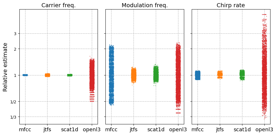
All feature representations are capable of regressing carrier frequency \(f_c\) with error ratios close to \(1\). However, larger performance discrepancies can be observed in modulation frequency and chirp rate. Time scattering and JTFS excel at linearizing modulation frequency in the Euclidean space, with error ratios within range of \(0.75\) to \(1.5\). Meanwhile, all scattering features extract chirp rate within error ratios between \(0.75\) to \(1.25\), while MFCCs fail to account for similarity in modulations.
We see that in the case of OpenL3, a significant portion of the regression targets are estimated by a factor of two or more for modulation frequency and chirp rate.